# 实现逻辑回归 对于这个秘籍，我们将实现逻辑回归来预测样本人群中低出生体重的概率。 ## 做好准备 逻辑回归是将线性回归转换为二元分类的一种方法。这是通过将线性输出转换为 Sigmoid 函数来实现的，该函数将输出在 0 和 1 之间进行缩放。目标是零或一，表示数据点是在一个类还是另一个类中。由于我们预测 0 和 1 之间的数字，如果预测高于指定的截止值，则预测被分类为类值 1，否则分类为 0。出于此示例的目的，我们将指定 cutoff 为 0.5，这将使分类像舍入输出一样简单。 我们将用于此示例的数据将是从作者的 GitHub 仓库获得的低出生体重数据（ [https://github.com/nfmcclure/tensorflow_cookbook/raw/master/01_Introduction/07_Working_with_Data_Sources/birthweight_data/birthweight.dat](https://github.com/nfmcclure/tensorflow_cookbook/raw/master/01_Introduction/07_Working_with_Data_Sources/birthweight_data/birthweight.dat) ）。我们将从其他几个因素预测低出生体重。 ## 操作步骤 我们按如下方式处理秘籍： 1. 我们首先加载库，包括`request`库，因为我们将通过超链接访问低出生体重数据。我们还发起了一个会议： ```py import matplotlib.pyplot as plt import numpy as np import tensorflow as tf import requests from sklearn import datasets from sklearn.preprocessing import normalize from tensorflow.python.framework import ops ops.reset_default_graph() sess = tf.Session() ``` 1. 接下来，我们通过请求模块加载数据并指定我们要使用的特征。我们必须具体，因为一个特征是实际出生体重，我们不想用它来预测出生体重是大于还是小于特定量。我们也不想将 ID 列用作预测器： ```py birth_weight_file = 'birth_weight.csv' # Download data and create data file if file does not exist in current directory if not os.path.exists(birth_weight_file): birthdata_url = 'https://github.com/nfmcclure/tensorflow_cookbook/raw/master/01_Introduction/07_Working_with_Data_Sources/birthweight_data/birthweight.dat' birth_file = requests.get(birthdata_url) birth_data = birth_file.text.split('\r\n') birth_header = birth_data[0].split('\t') birth_data = [[float(x) for x in y.split('\t') if len(x)>=1] for y in birth_data[1:] if len(y)>=1] with open(birth_weight_file, 'w', newline='') as f: writer = csv.writer(f) writer.writerow(birth_header) writer.writerows(birth_data) # Read birth weight data into memory birth_data = [] with open(birth_weight_file, newline='') as csvfile: csv_reader = csv.reader(csvfile) birth_header = next(csv_reader) for row in csv_reader: birth_data.append(row) birth_data = [[float(x) for x in row] for row in birth_data] # Pull out target variable y_vals = np.array([x[0] for x in birth_data]) # Pull out predictor variables (not id, not target, and not birthweight) x_vals = np.array([x[1:8] for x in birth_data]) ``` 1. 首先，我们将数据集拆分为测试和训练集： ```py train_indices = np.random.choice(len(x_vals), round(len(x_vals)*0.8), replace=False) test_indices = np.array(list(set(range(len(x_vals))) - set(train_indices))) x_vals_train = x_vals[train_indices] x_vals_test = x_vals[test_indices] y_vals_train = y_vals[train_indices] y_vals_test = y_vals[test_indices] ``` 1. 当特征在 0 和 1 之间缩放（最小 - 最大缩放）时，逻辑回归收敛效果更好。那么，接下来我们将扩展每个特征： ```py def normalize_cols(m, col_min=np.array([None]), col_max=np.array([None])): if not col_min[0]: col_min = m.min(axis=0) if not col_max[0]: col_max = m.max(axis=0) return (m-col_min) / (col_max - col_min), col_min, col_max x_vals_train, train_min, train_max = np.nan_to_num(normalize_cols(x_vals_train)) x_vals_test = np.nan_to_num(normalize_cols(x_vals_test, train_min, train_max)) ``` > 请注意，在缩放数据集之前，我们将数据集拆分为 train 和 test。这是一个重要的区别。我们希望确保测试集完全不影响训练集。如果我们在分裂之前缩放整个集合，那么我们不能保证它们不会相互影响。我们确保从训练组中保存缩放以缩放测试集。 1. 接下来，我们声明批量大小，占位符，变量和逻辑模型。我们不将输出包装在 sigmoid 中，因为该操作内置于 loss 函数中。另请注意，每次观察都有七个输入特征，因此`x_data`占位符的大小为`[None, 7]`。 ```py batch_size = 25 x_data = tf.placeholder(shape=[None, 7], dtype=tf.float32) y_target = tf.placeholder(shape=[None, 1], dtype=tf.float32) A = tf.Variable(tf.random_normal(shape=[7,1])) b = tf.Variable(tf.random_normal(shape=[1,1])) model_output = tf.add(tf.matmul(x_data, A), b) ``` 1. 现在，我们声明我们的损失函数，它具有 sigmoid 函数，初始化我们的变量，并声明我们的优化函数： ```py loss = tf.reduce_mean(tf.nn.sigmoid_cross_entropy_with_logits(model_output, y_target)) init = tf.global_variables_initializer() sess.run(init) my_opt = tf.train.GradientDescentOptimizer(0.01) train_step = my_opt.minimize(loss) ``` 1. 在记录损失函数的同时，我们还希望在训练和测试集上记录分类准确率。因此，我们将创建一个预测函数，返回任何大小的批量的准确率： ```py prediction = tf.round(tf.sigmoid(model_output)) predictions_correct = tf.cast(tf.equal(prediction, y_target), tf.float32) accuracy = tf.reduce_mean(predictions_correct) ``` 1. 现在，我们可以开始我们的训练循环并记录损失和准确率： ```py loss_vec = [] train_acc = [] test_acc = [] for i in range(1500): rand_index = np.random.choice(len(x_vals_train), size=batch_size) rand_x = x_vals_train[rand_index] rand_y = np.transpose([y_vals_train[rand_index]]) sess.run(train_step, feed_dict={x_data: rand_x, y_target: rand_y}) temp_loss = sess.run(loss, feed_dict={x_data: rand_x, y_target: rand_y}) loss_vec.append(temp_loss) temp_acc_train = sess.run(accuracy, feed_dict={x_data: x_vals_train, y_target: np.transpose([y_vals_train])}) train_acc.append(temp_acc_train) temp_acc_test = sess.run(accuracy, feed_dict={x_data: x_vals_test, y_target: np.transpose([y_vals_test])}) test_acc.append(temp_acc_test) ``` 1. 以下是查看损失和准确率图的代码： ```py plt.plot(loss_vec, 'k-') plt.title('Cross' Entropy Loss per Generation') plt.xlabel('Generation') plt.ylabel('Cross' Entropy Loss') plt.show() plt.plot(train_acc, 'k-', label='Train Set Accuracy') plt.plot(test_acc, 'r--', label='Test Set Accuracy') plt.title('Train and Test Accuracy') plt.xlabel('Generation') plt.ylabel('Accuracy') plt.legend(loc='lower right') plt.show() ``` ## 工作原理 这是迭代和训练和测试精度的损失。由于数据集仅为 189 次观测，因此随着数据集的随机分裂，训练和测试精度图将发生变化。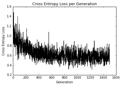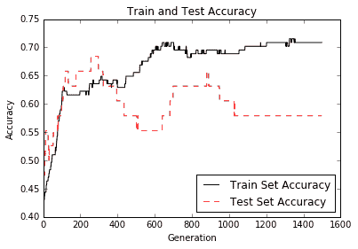第一个数字是交叉熵损失：  图 11：在 1,500 次迭代过程中绘制的交叉熵损失 第二个图显示了训练和测试装置的准确率： Figure 12: Test and train set accuracy plotted over 1,500 generations