# 为垃圾邮件预测实现 RNN 首先，我们将应用标准 RNN 单元来预测奇异数值输出，即垃圾邮件概率。 ## 做好准备 在此秘籍中，我们将在 TensorFlow 中实现标准 RNN，以预测短信是垃圾邮件还是火腿。我们将使用 UCI 的 ML 仓库中的 SMS 垃圾邮件收集数据集。我们将用于预测的架构将是来自嵌入文本的输入 RNN 序列，我们将最后的 RNN 输出作为垃圾邮件或火腿（1 或 0）的预测。 ## 操作步骤 1. 我们首先加载此脚本所需的库： ```py import os import re import io import requests import numpy as np import matplotlib.pyplot as plt import tensorflow as tf from zipfile import ZipFile ``` 1. 接下来，我们启动图会话并设置 RNN 模型参数。我们将通过`20`周期以`250`的批量大小运行数据。我们将考虑的每个文本的最大长度是`25`字;我们将更长的文本剪切为`25`或零填充短文本。 RNN 将是`10`单元。我们只考虑在词汇表中出现至少 10 次的单词，并且每个单词都将嵌入到可训练的大小`50`中。droupout 率将是我们可以在训练期间`0.5`或评估期间`1.0`设置的占位符： ```py sess = tf.Session() epochs = 20 batch_size = 250 max_sequence_length = 25 rnn_size = 10 embedding_size = 50 min_word_frequency = 10 learning_rate = 0.0005 dropout_keep_prob = tf.placeholder(tf.float32) ``` 1. 现在我们获取 SMS 文本数据。首先，我们检查它是否已经下载，如果是，请在文件中读取。否则，我们下载数据并保存： ```py data_dir = 'temp' data_file = 'text_data.txt' if not os.path.exists(data_dir): os.makedirs(data_dir) if not os.path.isfile(os.path.join(data_dir, data_file)): zip_url = 'http://archive.ics.uci.edu/ml/machine-learning-databases/00228/smsspamcollection.zip' r = requests.get(zip_url) z = ZipFile(io.BytesIO(r.content)) file = z.read('SMSSpamCollection') # Format Data text_data = file.decode() text_data = text_data.encode('ascii',errors='ignore') text_data = text_data.decode().split('\n') # Save data to text file with open(os.path.join(data_dir, data_file), 'w') as file_conn: for text in text_data: file_conn.write("{}\n".format(text)) else: # Open data from text file text_data = [] with open(os.path.join(data_dir, data_file), 'r') as file_conn: for row in file_conn: text_data.append(row) text_data = text_data[:-1] text_data = [x.split('\t') for x in text_data if len(x)>=1] [text_data_target, text_data_train] = [list(x) for x in zip(*text_data)] ``` 1. 为了减少我们的词汇量，我们将通过删除特殊字符和额外的空格来清理输入文本，并将所有内容放在小写中： ```py def clean_text(text_string): text_string = re.sub(r'([^sw]|_|[0-9])+', '', text_string) text_string = " ".join(text_string.split()) text_string = text_string.lower() return text_string # Clean texts text_data_train = [clean_text(x) for x in text_data_train] ``` > 请注意，我们的清洁步骤会删除特殊字符作为替代方案，我们也可以用空格替换它们。理想情况下，这取决于数据集的格式。 1. 现在我们使用 TensorFlow 的内置词汇处理器函数处理文本。这会将文本转换为适当的索引列表： ```py vocab_processor = tf.contrib.learn.preprocessing.VocabularyProcessor(max_sequence_length, min_frequency=min_word_frequency) text_processed = np.array(list(vocab_processor.fit_transform(text_data_train))) ``` > 请注意，`contrib.learn.preprocessing`中的函数目前已弃用（使用当前的 TensorFlow 版本，1.10）。目前的替换建议 TensorFlow 预处理包仅在 Python 2 中运行。将 TensorFlow 预处理移至 Python 3 的工作目前正在进行中，并将取代前两行。请记住，所有当前和最新的代码都可以在这个 GitHub 页面找到： [https://www.github.com/nfmcclure/tensorflow_cookbook](https://www.github.com/nfmcclure/tensorflow_cookbook) 和 Packt 仓库： [https：/ /github.com/PacktPublishing/TensorFlow-Machine-Learning-Cookbook-Second-Edition](https://github.com/PacktPublishing/TensorFlow-Machine-Learning-Cookbook-Second-Edition) 。 1. 接下来，我们将数据随机化以使其随机化： ```py text_processed = np.array(text_processed) text_data_target = np.array([1 if x=='ham' else 0 for x in text_data_target]) shuffled_ix = np.random.permutation(np.arange(len(text_data_target))) x_shuffled = text_processed[shuffled_ix] y_shuffled = text_data_target[shuffled_ix] ``` 1. 我们还将数据拆分为 80-20 训练测试数据集： ```py ix_cutoff = int(len(y_shuffled)*0.80) x_train, x_test = x_shuffled[:ix_cutoff], x_shuffled[ix_cutoff:] y_train, y_test = y_shuffled[:ix_cutoff], y_shuffled[ix_cutoff:] vocab_size = len(vocab_processor.vocabulary_) print("Vocabulary Size: {:d}".format(vocab_size)) print("80-20 Train Test split: {:d} -- {:d}".format(len(y_train), len(y_test))) ``` > 对于这个秘籍，我们不会进行任何超参数调整。如果读者朝这个方向前进，请记住在继续之前将数据集拆分为训练测试验证集。一个很好的选择是 Scikit-learn 函数`model_selection.train_test_split()`。 1. 接下来，我们声明图占位符。 `x`输入将是一个大小为`[None, max_sequence_length]`的占位符，它将是根据文本消息允许的最大字长的批量大小。对于火腿或垃圾邮件，`y` -output 占位符只是一个 0 或 1 的整数： ```py x_data = tf.placeholder(tf.int32, [None, max_sequence_length]) y_output = tf.placeholder(tf.int32, [None]) ``` 1. 我们现在为`x`输入数据创建嵌入矩阵和嵌入查找操作： ```py embedding_mat = tf.Variable(tf.random_uniform([vocab_size, embedding_size], -1.0, 1.0)) embedding_output = tf.nn.embedding_lookup(embedding_mat, x_data) ``` 1. 我们将模型声明如下。首先，我们初始化一种要使用的 RNN 小区（RNN 大小为 10）。然后我们通过使其成为动态 RNN 来创建 RNN 序列。然后我们将退出添加到 RNN： ```py cell = tf.nn.rnn_cell.BasicRNNCell(num_units = rnn_size) output, state = tf.nn.dynamic_rnn(cell, embedding_output, dtype=tf.float32) output = tf.nn.dropout(output, dropout_keep_prob) ``` > 注意，动态 RNN 允许可变长度序列。即使我们在这个例子中使用固定的序列长度，通常最好在 TensorFlow 中使用`dynamic_rnn`有两个主要原因。一个原因是，在实践中，动态 RNN 实际上运行速度更快;第二个是，如果我们选择，我们可以通过 RNN 运行不同长度的序列。 1. 现在要得到我们的预测，我们必须重新安排 RNN 并切掉最后一个输出： ```py output = tf.transpose(output, [1, 0, 2]) last = tf.gather(output, int(output.get_shape()[0]) - 1) ``` 1. 为了完成 RNN 预测，我们通过完全连接的网络层将`rnn_size`输出转换为两个类别输出： ```py weight = tf.Variable(tf.truncated_normal([rnn_size, 2], stddev=0.1)) bias = tf.Variable(tf.constant(0.1, shape=[2])) logits_out = tf.nn.softmax(tf.matmul(last, weight) + bias) ``` 1. 我们接下来宣布我们的损失函数。请记住，当使用 TensorFlow 中的`sparse_softmax`函数时，目标必须是整数索引（类型为`int`），并且 logits 必须是浮点数： ```py losses = tf.nn.sparse_softmax_cross_entropy_with_logits(logits=logits_out, labels=y_output) loss = tf.reduce_mean(losses) ``` 1. 我们还需要一个精确度函数，以便我们可以比较测试和训练集上的算法： ```py accuracy = tf.reduce_mean(tf.cast(tf.equal(tf.argmax(logits_out, 1), tf.cast(y_output, tf.int64)), tf.float32)) ``` 1. 接下来，我们创建优化函数并初始化模型变量： ```py optimizer = tf.train.RMSPropOptimizer(learning_rate) train_step = optimizer.minimize(loss) init = tf.global_variables_initializer() sess.run(init) ``` 1. 现在我们可以开始循环遍历数据并训练模型。在多次循环数据时，最好在每个周期对数据进行洗牌以防止过度训练： ```py train_loss = [] test_loss = [] train_accuracy = [] test_accuracy = [] # Start training for epoch in range(epochs): # Shuffle training data shuffled_ix = np.random.permutation(np.arange(len(x_train))) x_train = x_train[shuffled_ix] y_train = y_train[shuffled_ix] num_batches = int(len(x_train)/batch_size) + 1 for i in range(num_batches): # Select train data min_ix = i * batch_size max_ix = np.min([len(x_train), ((i+1) * batch_size)]) x_train_batch = x_train[min_ix:max_ix] y_train_batch = y_train[min_ix:max_ix] # Run train step train_dict = {x_data: x_train_batch, y_output: y_train_batch, dropout_keep_prob:0.5} sess.run(train_step, feed_dict=train_dict) # Run loss and accuracy for training temp_train_loss, temp_train_acc = sess.run([loss, accuracy], feed_dict=train_dict) train_loss.append(temp_train_loss) train_accuracy.append(temp_train_acc) # Run Eval Step test_dict = {x_data: x_test, y_output: y_test, dropout_keep_prob:1.0} temp_test_loss, temp_test_acc = sess.run([loss, accuracy], feed_dict=test_dict) test_loss.append(temp_test_loss) test_accuracy.append(temp_test_acc) print('Epoch: {}, Test Loss: {:.2}, Test Acc: {:.2}'.format(epoch+1, temp_test_loss, temp_test_acc)) ``` 1. 这导致以下输出： ```py Vocabulary Size: 933 80-20 Train Test split: 4459 -- 1115 Epoch: 1, Test Loss: 0.59, Test Acc: 0.83 Epoch: 2, Test Loss: 0.58, Test Acc: 0.83 ... ``` ```py Epoch: 19, Test Loss: 0.46, Test Acc: 0.86 Epoch: 20, Test Loss: 0.46, Test Acc: 0.86 ``` 1. 以下是绘制训练/测试损失和准确率的代码： ```py epoch_seq = np.arange(1, epochs+1) plt.plot(epoch_seq, train_loss, 'k--', label='Train Set') plt.plot(epoch_seq, test_loss, 'r-', label='Test Set') plt.title('Softmax Loss') plt.xlabel('Epochs') plt.ylabel('Softmax Loss') plt.legend(loc='upper left') plt.show() # Plot accuracy over time plt.plot(epoch_seq, train_accuracy, 'k--', label='Train Set') plt.plot(epoch_seq, test_accuracy, 'r-', label='Test Set') plt.title('Test Accuracy') plt.xlabel('Epochs') plt.ylabel('Accuracy') plt.legend(loc='upper left') plt.show() ``` ## 工作原理 在这个秘籍中，我们创建了一个 RNN 到类别的模型来预测 SMS 文本是垃圾邮件还是火腿。我们在测试装置上实现了大约 86％的准确率。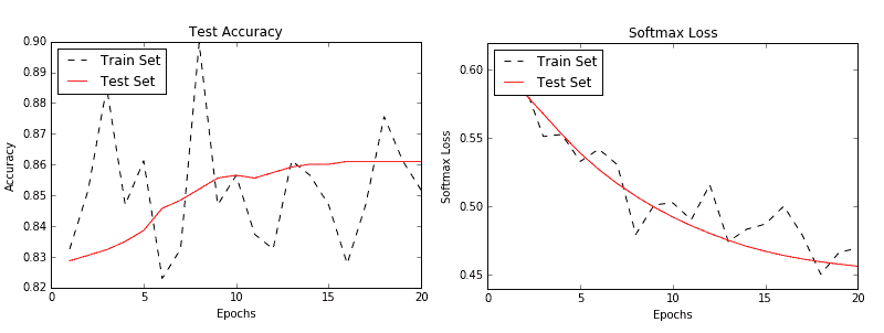以下是测试和训练集的准确率和损失图：  图 3：训练和测试集的准确率（左）和损失（右） ## 更多 强烈建议您多次浏览训练数据集以获取顺序数据（这也建议用于非顺序数据）。每次传递数据都称为周期。此外，在每个周期之前对数据进行混洗是非常常见的（并且强烈推荐），以最小化数据顺序对训练的影响。