# 使用最近邻 我们将通过实现最近邻来预测住房价值来开始本章。这是从最近邻居开始的好方法，因为我们将处理数字特征和连续目标。 ## 做好准备 为了说明如何在 TensorFlow 中使用最近邻居进行预测，我们将使用波士顿住房数据集。在这里，我们将预测邻域住房价值中位数作为几个特征的函数。 由于我们考虑训练集训练模型，我们将找到预测点的 k-NN，并将计算目标值的加权平均值。 ## 操作步骤 我们按如下方式处理秘籍： 1. 我们将从加载所需的库并开始图会话开始。我们将使用`requests`模块从 UCI 机器学习库加载必要的波士顿住房数据： ```py import matplotlib.pyplot as plt import numpy as np import tensorflow as tf import requests sess = tf.Session() ``` 1. 接下来，我们将使用`requests`模块加载数据： ```py housing_url = 'https://archive.ics.uci.edu/ml/machine-learning-databases/housing/housing.data' housing_header = ['CRIM', 'ZN', 'INDUS', 'CHAS', 'NOX', 'RM', 'AGE', 'DIS', 'RAD', 'TAX', 'PTRATIO', 'B', 'LSTAT', 'MEDV'] cols_used = ['CRIM', 'INDUS', 'NOX', 'RM', 'AGE', 'DIS', 'TAX', 'PTRATIO', 'B', 'LSTAT'] num_features = len(cols_used) # Request data housing_file = requests.get(housing_url) # Parse Data housing_data = [[float(x) for x in y.split(' ') if len(x)>=1] for y in housing_file.text.split('n') if len(y)>=1] ``` 1. 接下来，我们将数据分为依赖和独立的特征。我们将预测最后一个变量`MEDV`，这是房屋组的中值。我们也不会使用`ZN`，`CHAS`和`RAD`特征，因为它们没有信息或二元性质： ```py y_vals = np.transpose([np.array([y[13] for y in housing_data])]) x_vals = np.array([[x for i,x in enumerate(y) if housing_header[i] in cols_used] for y in housing_data]) x_vals = (x_vals - x_vals.min(0)) / x_vals.ptp(0) ``` 1. 现在，我们将`x`和`y`值分成训练和测试集。我们将通过随机选择大约 80％的行来创建训练集，并将剩下的 20％留给测试集： ```py train_indices = np.random.choice(len(x_vals), round(len(x_vals)*0.8), replace=False) test_indices = np.array(list(set(range(len(x_vals))) - set(train_indices))) x_vals_train = x_vals[train_indices] x_vals_test = x_vals[test_indices] y_vals_train = y_vals[train_indices] y_vals_test = y_vals[test_indices] ``` 1. 接下来，我们将声明`k`值和批量大小： ```py k = 4 batch_size=len(x_vals_test) ``` 1. 我们接下来会申报占位符。请记住，没有模型变量需要训练，因为模型完全由我们的训练集确定： ```py x_data_train = tf.placeholder(shape=[None, num_features], dtype=tf.float32) x_data_test = tf.placeholder(shape=[None, num_features], dtype=tf.float32) y_target_train = tf.placeholder(shape=[None, 1], dtype=tf.float32) y_target_test = tf.placeholder(shape=[None, 1], dtype=tf.float32) ``` 1. 接下来，我们将为一批测试点创建距离函数。在这里，我们将说明 L1 距离的使用： ```py distance = tf.reduce_sum(tf.abs(tf.subtract(x_data_train, tf.expand_dims(x_data_test,1))), reduction_indices=2) ``` > 注意，也可以使用 L2 距离函数。我们将距离公式改为`distance = tf.sqrt(tf.reduce_sum(tf.square(tf.subtract(x_data_train, tf.expand_dims(x_data_test,1))), reduction_indices=1))`。 1. 现在，我们将创建我们的预测函数。为此，我们将使用`top_k()`函数，该函数返回张量中最大值的值和索引。由于我们想要最小距离的指数，我们将找到`k` - 最大负距离。我们还将声明目标值的预测和均方误差（MSE）： ```py top_k_xvals, top_k_indices = tf.nn.top_k(tf.negative(distance), k=k) x_sums = tf.expand_dims(tf.reduce_sum(top_k_xvals, 1),1) x_sums_repeated = tf.matmul(x_sums,tf.ones([1, k], tf.float32)) x_val_weights = tf.expand_dims(tf.divide(top_k_xvals,x_sums_repeated), 1) top_k_yvals = tf.gather(y_target_train, top_k_indices) prediction = tf.squeeze(tf.batch_matmul(x_val_weights,top_k_yvals), squeeze_dims=[1]) mse = tf.divide(tf.reduce_sum(tf.square(tf.subtract(prediction, y_target_test))), batch_size) ``` 1. 现在，我们将遍历测试数据并存储预测和准确率值： ```py num_loops = int(np.ceil(len(x_vals_test)/batch_size)) for i in range(num_loops): min_index = i*batch_size max_index = min((i+1)*batch_size,len(x_vals_train)) x_batch = x_vals_test[min_index:max_index] y_batch = y_vals_test[min_index:max_index] predictions = sess.run(prediction, feed_dict={x_data_train: x_vals_train, x_data_test: x_batch, y_target_train: y_vals_train, y_target_test: y_batch}) batch_mse = sess.run(mse, feed_dict={x_data_train: x_vals_train, x_data_test: x_batch, y_target_train: y_vals_train, y_target_test: y_batch}) print('Batch #' + str(i+1) + ' MSE: ' + str(np.round(batch_mse,3))) Batch #1 MSE: 23.153 ``` 1. 另外，我们可以查看实际目标值与预测值的直方图。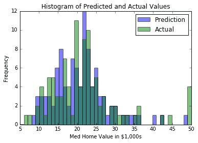看待这一点的一个原因是要注意这样一个事实：使用平均方法，我们无法预测目标的极端： ```py bins = np.linspace(5, 50, 45) plt.hist(predictions, bins, alpha=0.5, label='Prediction') plt.hist(y_batch, bins, alpha=0.5, label='Actual') plt.title('Histogram of Predicted and Actual Values') plt.xlabel('Med Home Value in $1,000s') plt.ylabel('Frequency') plt.legend(loc='upper right') plt.show() ``` 然后我们将获得直方图，如下所示：  图 1：k-NN 的预测值和实际目标值的直方图（其中`k=4`） 一个难以确定的是`k`的最佳价值。对于上图和预测，我们将`k=4`用于我们的模型。我们之所以选择这个，是因为它给了我们最低的 MSE。这通过交叉验证来验证。如果我们在`k`的多个值上使用交叉验证，我们将看到`k=4`给我们一个最小的 MSE。我们在下图中说明了这一点。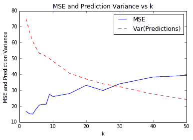绘制预测值的方差也是值得的，以表明它会随着我们平均的邻居越多而减少：  图 2：各种`k`值的 k-NN 预测的 MSE。我们还绘制了测试集上预测值的方差。请注意，随着`k`的增加，方差会减小。 ## 工作原理 使用最近邻算法，模型是训练集。因此，我们不必在模型中训练任何变量。唯一的参数`k`是通过交叉验证确定的，以最大限度地减少我们的 MSE。 ## 更多 对于 k-NN 的加权，我们选择直接按距离加权。还有其他选择我们也可以考虑。另一种常见方法是通过反平方距离加权。