# 实现先进的 CNN 能够扩展 CNN 模型以进行图像识别非常重要，这样我们才能理解如何增加网络的深度。如果我们有足够的数据，这可能会提高我们预测的准确率。扩展 CNN 网络的深度是以标准方式完成的：我们只是重复卷积，最大池和 ReLU，直到我们对深度感到满意为止。许多更精确的图像识别网络以这种方式操作。 ## 做好准备 在本文中，我们将实现一种更先进的读取图像数据的方法，并使用更大的 CNN 在 CIFAR10 数据集上进行图像识别（ [https://www.cs.toronto.edu/~kriz/cifar.html](https://www.cs.toronto.edu/~kriz/cifar.html) ）。该数据集具有 60,000 个`32x32`图像，这些图像恰好属于十个可能类别中的一个。图像的潜在类别是飞机，汽车，鸟，猫，鹿，狗，青蛙，马，船和卡车。另请参阅“另请参阅”部分中的第一个要点。 大多数图像数据集太大而无法放入内存中。我们可以使用 TensorFlow 设置一个图像管道，一次从一个文件中一次读取。我们通过设置图像阅读器，然后创建在图像阅读器上运行的批量队列来完成此操作。 此外，对于图像识别数据，通常在将图像发送之前随机扰动图像以进行训练。在这里，我们将随机裁剪，翻转和更改亮度。 此秘籍是官方 TensorFlow CIFAR-10 教程的改编版本，可在本章末尾的“另请参阅”部分中找到。我们将教程浓缩为一个脚本，我们将逐行完成并解释所有必要的代码。我们还将一些常量和参数恢复为原始引用的纸张值;我们将在适当的步骤中标记这一点。 ## 操作步骤 执行以下步骤： 1. 首先，我们加载必要的库并启动图会话： ```py import os import sys import tarfile import matplotlib.pyplot as plt import numpy as np import tensorflow as tf from six.moves import urllib sess = tf.Session() ``` 1. 现在我们将声明一些模型参数。我们的批量大小为 128（用于训练和测试）。我们将每 50 代输出一次状态，总共运行 20,000 代。每 500 代，我们将评估一批测试数据。然后我们将声明一些图像参数，高度和宽度，以及随机裁剪图像的大小。有三个通道（红色，绿色和蓝色），我们有十个不同的目标。然后我们将声明我们将从队列中存储数据和图像批次的位置： ```py batch_size = 128 output_every = 50 generations = 20000 eval_every = 500 image_height = 32 image_width = 32 crop_height = 24 crop_width = 24 num_channels = 3 num_targets = 10 data_dir = 'temp' extract_folder = 'cifar-10-batches-bin' ``` 1. 建议您在我们向好的模型迈进时降低学习率，因此我们将以指数方式降低学习率：初始学习率将设置为 0.1，并且我们将以 250％的指数方式将其降低 10％代。确切的公式将由`0.1 · 0.9^(x / 250)`给出，其中`x`是当前世代号。默认情况下，此值会持续降低，但 TensorFlow 会接受仅更新学习率的阶梯参数。这里我们设置一些参数供将来使用： ```py learning_rate = 0.1 lr_decay = 0.9 num_gens_to_wait = 250\. ``` 1. 现在我们将设置参数，以便我们可以读取二进制 CIFAR-10 图像： ```py image_vec_length = image_height * image_width * num_channels record_length = 1 + image_vec_length ``` 1. 接下来，我们将设置数据目录和 URL 以下载 CIFAR-10 图像，如果我们还没有它们： ```py data_dir = 'temp' if not os.path.exists(data_dir): os.makedirs(data_dir) cifar10_url = 'http://www.cs.toronto.edu/~kriz/cifar-10-binary.tar.gz' data_file = os.path.join(data_dir, 'cifar-10-binary.tar.gz') if not os.path.isfile(data_file): # Download file filepath, _ = urllib.request.urlretrieve(cifar10_url, data_file) # Extract file tarfile.open(filepath, 'r:gz').extractall(data_dir) ``` 1. 我们将设置记录阅读器并使用以下`read_cifar_files()`函数返回随机失真的图像。首先，我们需要声明一个读取固定字节长度的记录读取器对象。在我们读取图像队列之后，我们将图像和标签分开。最后，我们将使用 TensorFlow 的内置图像修改函数随机扭曲图像： ```py def read_cifar_files(filename_queue, distort_images = True): reader = tf.FixedLengthRecordReader(record_bytes=record_length) key, record_string = reader.read(filename_queue) record_bytes = tf.decode_raw(record_string, tf.uint8) # Extract label image_label = tf.cast(tf.slice(record_bytes, [0], [1]), tf.int32) # Extract image image_extracted = tf.reshape(tf.slice(record_bytes, [1], [image_vec_length]), [num_channels, image_height, image_width]) # Reshape image image_uint8image = tf.transpose(image_extracted, [1, 2, 0]) reshaped_image = tf.cast(image_uint8image, tf.float32) # Randomly Crop image final_image = tf.image.resize_image_with_crop_or_pad(reshaped_image, crop_width, crop_height) if distort_images: # Randomly flip the image horizontally, change the brightness and contrast final_image = tf.image.random_flip_left_right(final_image) final_image = tf.image.random_brightness(final_image,max_delta=63) final_image = tf.image.random_contrast(final_image,lower=0.2, upper=1.8) # Normalize whitening final_image = tf.image.per_image_standardization(final_image) return final_image, image_label ``` 1. 现在我们将声明一个函数，它将填充我们的图像管道以供批量器使用。我们首先需要设置一个我们想要读取的图像文件列表，并定义如何使用通过预构建的 TensorFlow 函数创建的输入生成器对象来读取它们。输入生成器可以传递给我们在上一步中创建的读取函数：`read_cifar_files()`。然后我们将在队列中设置批量阅读器：`shuffle_batch()`： ```py def input_pipeline(batch_size, train_logical=True): if train_logical: files = [os.path.join(data_dir, extract_folder, 'data_batch_{}.bin'.format(i)) for i in range(1,6)] else: files = [os.path.join(data_dir, extract_folder, 'test_batch.bin')] filename_queue = tf.train.string_input_producer(files) image, label = read_cifar_files(filename_queue) min_after_dequeue = 1000 capacity = min_after_dequeue + 3 * batch_size example_batch, label_batch = tf.train.shuffle_batch([image, label], batch_size, capacity, min_after_dequeue) return example_batch, label_batch ``` > 正确设置`min_after_dequeue`很重要。此参数负责设置用于采样的图像缓冲区的最小大小。官方 TensorFlow 文档建议将其设置为`(#threads + error margin)*batch_size`。请注意，将其设置为更大的大小会导致更均匀的混洗，因为它正在从队列中的更大数据集进行混洗，但是在此过程中也将使用更多内存。 1. 接下来，我们可以声明我们的模型函数。我们将使用的模型有两个卷积层，后面是三个完全连接的层。为了使变量声明更容易，我们首先声明两个变量函数。两个卷积层将分别创建 64 个特征。第一个完全连接的层将第二个卷积层与 384 个隐藏节点连接起来。第二个完全连接的操作将这 384 个隐藏节点连接到 192 个隐藏节点。最后的隐藏层操作将 192 个节点连接到我们试图预测的 10 个输出类。请参阅以下`#`前面的内联注释： ```py def cifar_cnn_model(input_images, batch_size, train_logical=True): def truncated_normal_var(name, shape, dtype): return tf.get_variable(name=name, shape=shape, dtype=dtype, initializer=tf.truncated_normal_initializer(stddev=0.05)) def zero_var(name, shape, dtype): return tf.get_variable(name=name, shape=shape, dtype=dtype, initializer=tf.constant_initializer(0.0)) # First Convolutional Layer with tf.variable_scope('conv1') as scope: # Conv_kernel is 5x5 for all 3 colors and we will create 64 features conv1_kernel = truncated_normal_var(name='conv_kernel1', shape=[5, 5, 3, 64], dtype=tf.float32) # We convolve across the image with a stride size of 1 conv1 = tf.nn.conv2d(input_images, conv1_kernel, [1, 1, 1, 1], padding='SAME') # Initialize and add the bias term conv1_bias = zero_var(name='conv_bias1', shape=[64], dtype=tf.float32) conv1_add_bias = tf.nn.bias_add(conv1, conv1_bias) # ReLU element wise relu_conv1 = tf.nn.relu(conv1_add_bias) # Max Pooling pool1 = tf.nn.max_pool(relu_conv1, ksize=[1, 3, 3, 1], strides=[1, 2, 2, 1],padding='SAME', name='pool_layer1') # Local Response Normalization norm1 = tf.nn.lrn(pool1, depth_radius=5, bias=2.0, alpha=1e-3, beta=0.75, name='norm1') # Second Convolutional Layer with tf.variable_scope('conv2') as scope: # Conv kernel is 5x5, across all prior 64 features and we create 64 more features conv2_kernel = truncated_normal_var(name='conv_kernel2', shape=[5, 5, 64, 64], dtype=tf.float32) # Convolve filter across prior output with stride size of 1 conv2 = tf.nn.conv2d(norm1, conv2_kernel, [1, 1, 1, 1], padding='SAME') # Initialize and add the bias conv2_bias = zero_var(name='conv_bias2', shape=[64], dtype=tf.float32) conv2_add_bias = tf.nn.bias_add(conv2, conv2_bias) # ReLU element wise relu_conv2 = tf.nn.relu(conv2_add_bias) # Max Pooling pool2 = tf.nn.max_pool(relu_conv2, ksize=[1, 3, 3, 1], strides=[1, 2, 2, 1], padding='SAME', name='pool_layer2') # Local Response Normalization (parameters from paper) norm2 = tf.nn.lrn(pool2, depth_radius=5, bias=2.0, alpha=1e-3, beta=0.75, name='norm2') # Reshape output into a single matrix for multiplication for the fully connected layers reshaped_output = tf.reshape(norm2, [batch_size, -1]) reshaped_dim = reshaped_output.get_shape()[1].value # First Fully Connected Layer with tf.variable_scope('full1') as scope: # Fully connected layer will have 384 outputs. full_weight1 = truncated_normal_var(name='full_mult1', shape=[reshaped_dim, 384], dtype=tf.float32) full_bias1 = zero_var(name='full_bias1', shape=[384], dtype=tf.float32) full_layer1 = tf.nn.relu(tf.add(tf.matmul(reshaped_output, full_weight1), full_bias1)) # Second Fully Connected Layer with tf.variable_scope('full2') as scope: # Second fully connected layer has 192 outputs. full_weight2 = truncated_normal_var(name='full_mult2', shape=[384, 192], dtype=tf.float32) full_bias2 = zero_var(name='full_bias2', shape=[192], dtype=tf.float32) full_layer2 = tf.nn.relu(tf.add(tf.matmul(full_layer1, full_weight2), full_bias2)) # Final Fully Connected Layer -> 10 categories for output (num_targets) with tf.variable_scope('full3') as scope: # Final fully connected layer has 10 (num_targets) outputs. full_weight3 = truncated_normal_var(name='full_mult3', shape=[192, num_targets], dtype=tf.float32) full_bias3 = zero_var(name='full_bias3', shape=[num_targets], dtype=tf.float32) final_output = tf.add(tf.matmul(full_layer2, full_weight3), full_bias3) return final_output ``` > 我们的本地响应标准化参数取自本文，并在本文的“另请参见”部分中引用。 1. 现在我们将创建损失函数。我们将使用 softmax 函数，因为图片只能占用一个类别，因此输出应该是十个目标的概率分布： ```py def cifar_loss(logits, targets): # Get rid of extra dimensions and cast targets into integers targets = tf.squeeze(tf.cast(targets, tf.int32)) # Calculate cross entropy from logits and targets cross_entropy = tf.nn.sparse_softmax_cross_entropy_with_logits(logits=logits, labels=targets) # Take the average loss across batch size cross_entropy_mean = tf.reduce_mean(cross_entropy) return cross_entropy_mean ``` 1. 接下来，我们宣布我们的训练步骤。学习率将以指数阶跃函数降低： ```py def train_step(loss_value, generation_num): # Our learning rate is an exponential decay (stepped down) model_learning_rate = tf.train.exponential_decay(learning_rate, generation_num, num_gens_to_wait, lr_decay, staircase=True) # Create optimizer my_optimizer = tf.train.GradientDescentOptimizer(model_learning_rate) # Initialize train step train_step = my_optimizer.minimize(loss_value) return train_step ``` 1. 我们还必须具有精确度函数，以计算一批图像的准确率。我们将输入 logits 和目标向量，并输出平均精度。然后我们可以将它用于训练和测试批次： ```py def accuracy_of_batch(logits, targets): # Make sure targets are integers and drop extra dimensions targets = tf.squeeze(tf.cast(targets, tf.int32)) # Get predicted values by finding which logit is the greatest batch_predictions = tf.cast(tf.argmax(logits, 1), tf.int32) # Check if they are equal across the batch predicted_correctly = tf.equal(batch_predictions, targets) # Average the 1's and 0's (True's and False's) across the batch size accuracy = tf.reduce_mean(tf.cast(predicted_correctly, tf.float32)) return accuracy ``` 1. 现在我们有了一个图像管道函数，我们可以初始化训练图像管道和测试图像管道： ```py images, targets = input_pipeline(batch_size, train_logical=True) test_images, test_targets = input_pipeline(batch_size, train_logical=False) ``` 1. 接下来，我们将初始化训练输出和测试输出的模型。值得注意的是，我们必须在创建训练模型后声明`scope.reuse_variables()`，这样，当我们为测试网络声明模型时，它将使用相同的模型参数： ```py with tf.variable_scope('model_definition') as scope: # Declare the training network model model_output = cifar_cnn_model(images, batch_size) # Use same variables within scope scope.reuse_variables() # Declare test model output test_output = cifar_cnn_model(test_images, batch_size) ``` 1. 我们现在可以初始化我们的损耗和测试精度函数。然后我们将声明`generation`变量。此变量需要声明为不可训练，并传递给我们的训练函数，该函数在学习率指数衰减计算中使用它： ```py loss = cifar_loss(model_output, targets) accuracy = accuracy_of_batch(test_output, test_targets) generation_num = tf.Variable(0, trainable=False) train_op = train_step(loss, generation_num) ``` 1. 我们现在将初始化所有模型的变量，然后通过运行 TensorFlow 函数`start_queue_runners()`来启动图像管道。当我们开始训练或测试模型输出时，管道将输入一批图像来代替饲料字典： ```py init = tf.global_variables_initializer() sess.run(init) tf.train.start_queue_runners(sess=sess) ``` 1. 我们现在循环训练我们的训练，节省训练损失和测试准确率： ```py train_loss = [] test_accuracy = [] for i in range(generations): _, loss_value = sess.run([train_op, loss]) if (i+1) % output_every == 0: train_loss.append(loss_value) output = 'Generation {}: Loss = {:.5f}'.format((i+1), loss_value) print(output) if (i+1) % eval_every == 0: [temp_accuracy] = sess.run([accuracy]) test_accuracy.append(temp_accuracy) acc_output = ' --- Test Accuracy= {:.2f}%.'.format(100\. * temp_accuracy) print(acc_output) ``` 1. 这导致以下输出： ```py ... Generation 19500: Loss = 0.04461 --- Test Accuracy = 80.47%. Generation 19550: Loss = 0.01171 Generation 19600: Loss = 0.06911 Generation 19650: Loss = 0.08629 Generation 19700: Loss = 0.05296 Generation 19750: Loss = 0.03462 Generation 19800: Loss = 0.03182 Generation 19850: Loss = 0.07092 Generation 19900: Loss = 0.11342 Generation 19950: Loss = 0.08751 Generation 20000: Loss = 0.02228 --- Test Accuracy = 83.59%. ``` 1. 最后，这里有一些`matplotlib`代码将绘制在训练过程中的损失和测试准确率： ```py eval_indices = range(0, generations, eval_every) output_indices = range(0, generations, output_every) # Plot loss over time plt.plot(output_indices, train_loss, 'k-') plt.title('Softmax Loss per Generation') plt.xlabel('Generation') plt.ylabel('Softmax Loss') plt.show() # Plot accuracy over time plt.plot(eval_indices, test_accuracy, 'k-') plt.title('Test Accuracy') plt.xlabel('Generation') plt.ylabel('Accuracy') plt.show() ``` 我们得到以下秘籍的以下绘图：  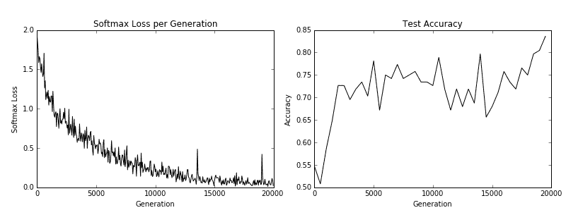图 5：训练损失在左侧，测试精度在右侧。对于 CIFAR-10 图像识别 CNN，我们能够实现在测试集上达到约 75％准确率的模型 ## 工作原理 在我们下载了 CIFAR-10 数据之后，我们建立了一个图像管道而不是使用源字典。有关图像管道的更多信息，请参阅官方 TensorFlow CIFAR-10 教程。我们使用此训练和测试管道来尝试预测图像的正确类别。最后，该模型在测试集上达到了约 75％的准确率。 ## 另见 * 有关 CIFAR-10 数据集的更多信息，请参阅学习 Tiny Images 的多个特征层，Alex Krizhevsky，2009： [https://www.cs.toronto.edu/~kriz/learning-features-2009- TR.pdf](https://www.cs.toronto.edu/~kriz/learning-features-2009-TR.pdf) * 要查看原始的 TensorFlow 代码，请参阅： [https://github.com/tensorflow/models/tree/master/tutorials/image/cifar10](https://github.com/tensorflow/models/tree/master/tutorials/image/cifar10) * 有关局部响应归一化的更多信息，请参阅使用深度卷积神经网络的 ImageNet 分类，Krizhevsky，A。等。人。 2012： [http://papers.nips.cc/paper/4824-imagenet-classification-with-deep-convolutional-neural-networks](http://papers.nips.cc/paper/4824-imagenet-classification-with-deep-convolutional-neural-networks)