# 二分类 二分类是指仅有两个不同类的问题。正如我们在上一章中所做的那样，我们将使用 SciKit Learn 库中的便捷函数`make_classification()`生成数据集： ```py X, y = skds.make_classification(n_samples=200, n_features=2, n_informative=2, n_redundant=0, n_repeated=0, n_classes=2, n_clusters_per_class=1) if (y.ndim == 1): y = y.reshape(-1,1) ``` `make_classification()`的论据是不言自明的; `n_samples`是要生成的数据点数，`n_features`是要生成的特征数，`n_classes`是类的数量，即 2： * `n_samples`是要生成的数据点数。我们将其保持在 200 以保持数据集较小。 * `n_features`是要生成的特征数量;我们只使用两个特征，因此我们可以将它作为一个简单的问题来理解 TensorFlow 命令。 * `n_classes`是类的数量，它是 2，因为它是二分类问题。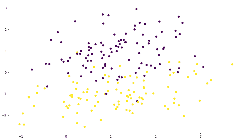 让我们使用以下代码绘制数据： ```py plt.scatter(X[:,0],X[:,1],marker='o',c=y) plt.show() ``` 我们得到以下绘图;您可能会得到一个不同的图，因为每次运行数据生成函数时都会随机生成数据：  然后我们使用 NumPy `eye`函数将`y`转换为单热编码目标： ```py print(y[0:5]) y=np.eye(num_outputs)[y] print(y[0:5]) ``` 单热编码目标如下所示： ```py [1 0 0 1 0] [[ 0\. 1.] [ 1\. 0.] [ 1\. 0.] [ 0\. 1.] [ 1\. 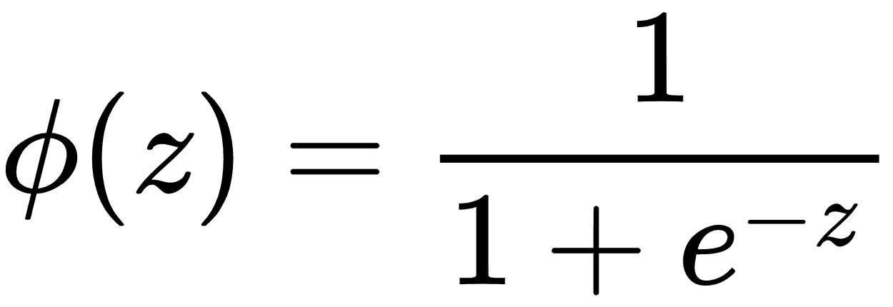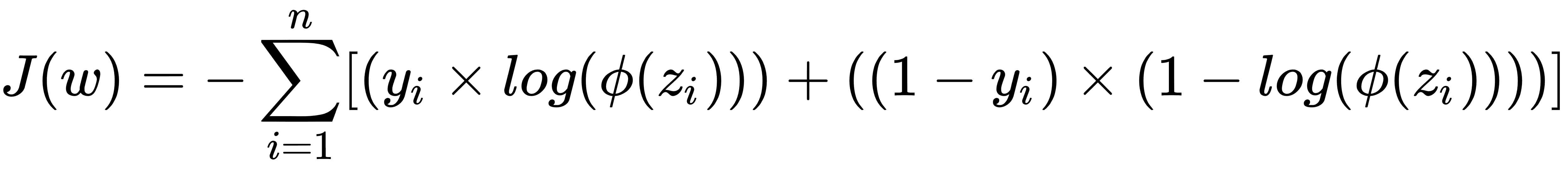0.]] ``` 将数据划分为训练和测试类别： ```py X_train, X_test, y_train, y_test = skms.train_test_split( X, y, test_size=.4, random_state=42) ``` 在分类中，我们使用 sigmoid 函数来量化模型的值，使得输出值位于范围[0,1]之间。以下等式表示由`φ(z)`表示的 S 形函数，其中`z`是等式`w × x + b`。损失函数现在变为由`J(θ)`表示的值，其中`θ`表示参数。    我们使用以下代码实现新模型和损失函数： ```py num_outputs = y_train.shape[1] num_inputs = X_train.shape[1] learning_rate = 0.001 # input images x = tf.placeholder(dtype=tf.float32, shape=[None, num_inputs], name="x") # output labels y = tf.placeholder(dtype=tf.float32, shape=[None, num_outputs], name="y") # model paramteres w = tf.Variable(tf.zeros([num_inputs,num_outputs]), name="w") b = tf.Variable(tf.zeros([num_outputs]), name="b") model = tf.nn.sigmoid(tf.matmul(x, w) + b) loss = tf.reduce_mean(-tf.reduce_sum( (y * tf.log(model)) + ((1 - y) * tf.log(1 - model)), axis=1)) optimizer = tf.train.GradientDescentOptimizer( learning_rate=learning_rate).minimize(loss) ``` 最后，我们运行我们的分类模型： ```py num_epochs = 1 with tf.Session() as tfs: tf.global_variables_initializer().run() for epoch in range(num_epochs): tfs.run(optimizer, feed_dict={x: X_train, y: y_train}) y_pred = tfs.run(tf.argmax(model, 1), feed_dict={x: X_test}) y_orig = tfs.run(tf.argmax(y, 1), feed_dict={y: y_test}) preds_check = tf.equal(y_pred, y_orig) accuracy_op = tf.reduce_mean(tf.cast(preds_check, tf.float32)) accuracy_score = tfs.run(accuracy_op) print("epoch {0:04d} accuracy={1:.8f}".format( epoch, accuracy_score)) plt.figure(figsize=(14, 4)) plt.subplot(1, 2, 1) plt.scatter(X_test[:, 0], X_test[:, 1], marker='o', c=y_orig) plt.title('Original') plt.subplot(1, 2, 2) plt.scatter(X_test[:, 0], X_test[:, 1], marker='o', c=y_pred) plt.title('Predicted') plt.show() ``` 我们获得了大约 96%的相当好的准确率，原始和预测的数据图如下所示：  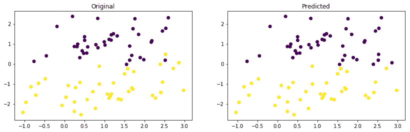很简约！！现在让我们让我们的问题变得复杂，并尝试预测两个以上的类。